Let’s quickly outline the idea behind the trading bot that we will be implementing in this video. This is just a simple trading bot for the sake of practice, please do not expect to build a trading bot that you would want to fund with your actual real money.

The ide behind this bot will be to buy and hold SPY which is the ETF for the S&P 500 Index.

To make things more interesting, we will want to close our position, if it loses more than 10% or if it climbs more than 10%.

After this we stop investing for a predetermined period of time such as one month.

Let’s Get Started Writing Code

Go to quantconnect.com and click on Algorithm Lab

Click the Create New Algorithm button

It will load a coding IDE for you and start you on a file main.py with some boilerplate already in there for you.

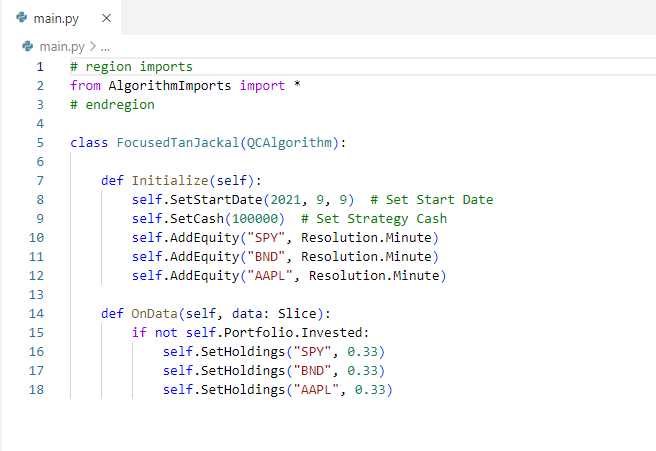
The initialize function will be called once at the beginning of your algorithm and you will use it for setup.

The OnData function is called every time a tick or data bar reaches its end time as the Time Frontier moves through time.

The time frontier is basically a variable indicating the “current time”. You can travel through historical time when backtesting your algorithm for example, and this time frontier just travels through the alotted time period marking the current time.

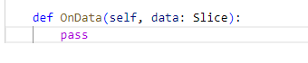
Let’s set OnData to be empty, we will get back to that function later,

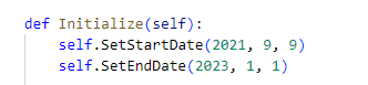
and then the first thing we will do is set a start and end date for our backtesting. If you don’t specify an end date, the most recent date will be chosen.

Next, we will set the starting cash balance for the algo.

Once again, this is just for backtesting purposes. In real life trading, this number will be taken from your brokerage account balance.

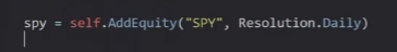
Next we will add data about the ETF that we want to trade. We will use the SPY ticker to trade equities on the S&P 500, and specify that we want to use daily time bars. This argument is referred to as the time resolution. The lowest resolution available is the tick resolution can be as low as a tick per millisecond. Note that such a low resolution will lead to a large number of data points which will be hard to process efficiently. Daily will suffice for our algorithm. Moreover, tick data is raw and unfiltered which can lead to unwanted problems. In general, if you’re not completely sure of what you’re doing, it’s recommended not to go below minute resolution.

Data Normalization Mode

Next we will set the data normalization mode for our SPY equity data. QuantConnect supports 4 data normalization modes.

The default data adjustment mode is split and dividend adjusted. This means that the data is smoothed out so that the stock splits don’t look like huge drops or spikes. This can be very useful and make the data easier to handle.

What Is an Equity Split?

Equity refers to non cash compensation that represents partial ownership in a company. The equity is usually split up or divided among early founders, financial supporters, and sometimes employees who join the startup in its earliest stages.

Raw data is not adjusted. Dividends are paid in cash and the stock’s price is not adjusted. Certain assets classes such as options can only be used with raw data.

We are going to set the data normalization mode to raw.

spy.SetDataNormalizationMode(DataNormalizationMode.Raw)

Note that a lot of times you will not need to change the data normalization mode since you can just use the default mode, but nonetheless it is good to know how to do so.

next, let’s set the spy variable to be a symbol object and store it in self.

 self.spy = spy.Symbol

If you’re not familiar with symbol objects in QuantConnect, I recommended reading this tutorial:

After saving the symbol object let’s set a bench mark for this algo:

self.SetBenchmark("SPY")

Since we’re trading SPY, we’ll just use SPY as the benchmark. Here you’ll want to compare your algorithm against some common market index in the traded sector.

QC also allows you to set for different brokerage models to account for your brokers fee structure and account type. The default brokerage model is usually good enough but you can also specify the Interactive Brokers brokerage model, FXCM brokers, BitFinex and so on if you want to.

Besides setting the broker type you can set the account type to a cash or a margin account.

self.SetBrokerageModel(BrokerageName.InteractiveBrokersBrokerage, Accounttype.Margin)

a cash account does not allow you to use leverage and it has a settling period of 3 days for equities. We are using a margin account but this algorithm could also easily be used for a cash account. Usually with cash accounts you just need to be careful about the t+3 settlement rules.

Last but not least we will create 3 custom helper variables. First we will create the entry price, which will set the entry price of our SPY position.

self.entryPrice = 0

the second is self.period which we will set to a time frame of 31 days.

self.period = timedelta(31)

and finally self.nextEntryTime which will track when we will reenter a long SPY position. We will set this to the current time since we want to start investing right away.

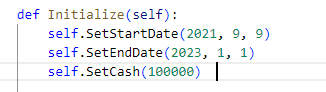
self.nextEntryTime = self.Time

Now we are finally done with the initialization method, here is the entire code snipped for the initialization method.

def Initialize(self):
        self.SetStartDate(2021, 9, 9) 
        self.SetEndDate(2023, 1, 1)
        self.SetCash(100000)  
        self.AddEquity("SPY", Resolution.Daily)
        spy.SetDataNormalizationMode(DataNormalizationMode.Raw)
        self.spy = spy.Symbol
        self.SetBenchmark("SPY")
        self.SetBrokerageModel(BrokerageName.InteractiveBrokersBrokerage, Accounttype.Margin)

        self.entryPrice = 0
        self.period = timedelta(31)
        self.nextEntryTime = self.Time

now we can start implementing the OnData method. Remember this is called every time the end of a bar is reached or a tick has occurred.

Notice that the OnData method has only one parameter called data.

def OnData(self, data: Slice):
        pass

The data parameter is a Slice object that is passed to the OnData event handler as previously explained every time a tick occurs or the end of a time bar is reached.

The Slice object provides you with a bunch of helpers for handling data. Please see the picture above with the class definition.

These items are dictionaries that are referenced by symbols.

Let’s walk through the data type of the most significant of these objects. These types all extend the BaseData data type which provides you with symbol, value (ticker symbol) and time information.

Let us first discuss Ticks. The most interesting piece of Tick data is the LastPrice

but as mentioned before, Tick data is raw and unfiltered.

The next important data type is trade bars. Since this trade bar data covers a period of time it is passed to it’s event handler at it’s end time.

Trade bars are supported for equities, options and futures. It provides you with open, high, low, and close information.

TradeBars are built from consolidating trades from exchanges.

Note that we will go over more about TradeBars in a minute, but first I will finish going over these Slice data helper objects on a conceptual level.

The next data type is QuoteBars

QuoteBars are supported by all asset types so also by Forex, cryptos, and CFDs.

The main difference between QuoteBars and TradeBars is that QuoteBars are built from consolidating bid price and the ask price from exchanges. QuoteBars are for open, high, low, close, bid, ask, lastBidSize and lastAskSize properties. Here the bid ask objects are bard themselves, which include properties open, high, low, and close info. The open, high, low and close info from the Quote bars, are generated from the midpoint of the bid and ask bars.

Now that we have a good grasp on the theory of the items in the data object, let’s start implementing the OnData method.

First we will save the current price of the SPY into a variable named price.

There are multiple ways of accomplishing this.

The first would be to access the bars of the data slice object. data.Bars is a dictionary which we can pass the value of self.spy which is a symbol object for the SPY index we set up in the initialize function. Since we want the most recent price, we will save the Close price. Note that this will be the closing price of the day before, since we don’t know yet what today’s closing price will be.

def OnData(self, data: Slice):
        price = data.Bars[self.spy].Close

Another way to accomplish the same thing would be to directly access the data variable. This would also return a bar that could be used to access the last Close price of yesterdays bar.

price = data[self.spy].Close

a third way to achieve the same result would be to use the self.Securities dictionary. We can then index self.Securities by the symbol and then save the closing price.

price = self.Securities[self.spy].Close

when using slice to access data, it can be useful to see if the requested data, does already exist.

If you just added the data, or there hasn’t been a lot of trading activity, your algorithm might not have access to the symbol yet.

To test if a symbol exists yet, you can use the contains function on a dictionary, or use the in keyword in python to see if the requested symbol is in data yet.

def OnData(self, data: Slice):
  if not self.spy in data:
    return

  price = data[self.spy].Close

Since SPY is very actively and we aren’t dynamically adding any data, this won’t make a difference for this example, but it is good to know how to do nonetheless.

next lets implement the trade logic of our bot. First we will check if our bot is already invested. We can do this, with self.Portfolio.invested which will return a boolean. It is also possible to check the Portfolio for a specific symbol and check if we are invested specifically, but since we are only trading SPY, this won’t be necessary here.

if not self.Portfolio.Invested:
  pass

Besides checking if we are invested, we can also check any of these popular values in Portfolio:

If we are not invested, we want to check if it is time to invest. As a reminder, this bot is supposed to buy and hold SPY until SPY drops 10% or rises 10%. Thereafter, we will stay in cash for one month, whereafter we will buy and hold again.

To account for the waiting period, we can check if the self.nextEntryTime is greater than or equal to the current time, if this is fulfilled, we want to buy as much SPY as we can. We can buy SPY using self.MarketOrder which sends a market order for the specified symbol and quantity. We will use int() to make all values round to the nearest integer. We will divide the number in Portfolio.Cash (all the cash we have available) by the price of an entry in SPY to order the max number of entries we can afford.

if not self.Portfolio.Invested: 
  if self.nextEntryTime <= self.Time:
    self.MarketOrder(self.spy, int(self.Portfolio.Cash / price))

a short hand way of achieving the same thing is to use SetHoldings. We can pass self.spy, and 1 indicate that we want to allocate 100% of our holdings to purchasing SPY.

if not self.Portfolio.Invested:
  if self.nextEntryTime <= self.Time:
    self.SetHoldings(self.spy, 1)

After this we want to log that we just bought SPY at the current price. Logging our actions can be very helpful when you are reviewing and debugging your algorithm. Also we will set the entry price to the new price that we just bought at.

self.Log("Buy SPY @" + str(price))
self.entryPrice = price

next we will set the other half of the if else condition. First we check:

if not self.Portfolio.Invested:

next let’s say we are invested, ie we are holding some stocks from SPY, we will check next if the price has gone down 10% or up 10% from our current position.

elif self.entryPrice * 1.1 < price or self.entryPrice * 0.9 > price:

if that condition is met, we want to sell all of our position, which is also called Liquidating.

self.Liquidate()

alternatively you can pass in the symbol that you want to liquidate for if you don’t want to liquidate your entire portfolio. (Note: that means we sell all our holdings)

self.Liquidate(self.spy)

now we will log that we closed our SPY position.

elif self.entryPrice * 1.1 < price or self.entryPrice * 0.9 > price: 
  self.Liquidate()
  self.Log("SELL SPY @" + str(price))

now we will wait for the next 30 days

self.nextEntryTime = self.time + self.period

heres the complete OnData function

def OnData(self, data: Slice):
  if not self.spy in data:
    return

  price = data[self.spy].Close

if not self.Portfolio.Invested:
    if self.nextEntryTime <= self.Time:
      self.SetHoldings(self.spy, 1)
      self.Log("Buy SPY @" + str(price))

elif self.entryPrice * 1.1 < price or self.entryPrice * 0.9 > price:
    self.Liquidate()
    self.Log("Sell SPY @" + str(price))
    self.nextEntryTime = self.Time + self.period

Now we will build and click the backtest button, which will show us how this algorithm would have performed over the specified time frame.

Analytics dashboard view like this one will be generated.

This equity chart will show your strategy’s performance. On this chart you can clearly see the flat line periods where our algorithm had a break from investing.

Above this chart are some stats for total profit, total fees and more.

In the top right corner you can select which charts you want to be displayed.

The benchmark box will be most interesting, as it will show us the comparison of how our algorithm compared to the performance of SPY.

Of most interest to us will be the benchmark chart.

Our algorithm is very highly correlated with the performance of SPY, so it is likely that this algorithm will not perform well in bear markets.

At the bottom are more useful stats that can be used to analyze your strategy’s performance.

There is also a logs tab which shows you all the generated logs from your algorithm.

This is not a good trading strategy or a useful bot, this is just a code example to display for educational purposes for learning to code in QuantConnect.